Feature Engineering by Example

It has happened to me one or the other time that I could not reproduce the results of scientific publications. Sometimes it was simply because important details in the algorithms used were either accidental or deliberately inaccurate. Sometimes, however, it was something else. The authors focused on a particular part of the processing pipeline, such as a particular algorithm of machine learning. However, another important part was omitted. How was the data pre-processed for the algorithm? What was the actual input into an artificial neuronal network?

In this article, I will give examples of what you can do with raw data before it is further processed.

Data & Goal

I’ll use the data from the LID-DS (Leipzig Intrusion Detection – Data Set) [LID-DS]. It is a modern host based intrusion detection system (HIDS) data set, containing system calls with their metadata like parameters, return values, user ids, process/thread ids, file system handles, timestamps, and io buffers.

To keep the example for this article as small as possible, I will only use a small part from the CVE-2012-2122 scenario. Simply said, the scenario [Source at GitHub] consists of a MySQL server in a certain version. Multiple users connect to the database and either add different words to the database or query individual random words. The attacker in this scenario uses the fact that MySQL and MariaDB of certain versions, „when running in certain environments with certain implementations of the memcmp function, allows remote attackers tobypass authentication by repeatedly authenticating with the same incorrect password, which eventually causes a token comparison to succeed due to an improperly-checked return value.“ [Common Vulnerabilities and Exposures]

For the following examples I will only use the frequency of system calls as input data. Please note that this may not be a good feature. To keep the example small I used only 50 sequences with normal and 50 sequences with attack behaviour as training data and the same amount of data for validation. I used a system call table with 520 entries to map each system call to a uniqe number, therefore the feature (frequency of system calls in sequence) has 520 dimensions, of which many are never actually used, but „I don’t know that yet at this point“.

One sequence of the used data looks like this one:

name_of_sequence 373 370 518 370 103 ... 415 321 321 84 84 321 518 # sequences variable in length

To calculate the feature vector for a sequence, I simply counted how often each system call occurs within the sequence and got a result like:

[0, 0, 0, 12, 0, 26, 0, 0, 0, 0, 0, ... 0, 0, 696, 0, 834, 11] # length = 520

The goal for the following examples is to classify the data into two classes: normal bahaviour and attack behaviour.

Visualization of the Input Data

This animation shows the feature „frequency of system calls in sequence“ for all training sequences. This includes normal behaviour sequences and attack behaviour sequences. Can you spot the normal and/or the attack vectors?

SVM with Raw Data

At first I tried to feed the „raw data“ (the unmodified feature vectors) into a SVM (Support Vector Machine).

from sklearn import svm
# training data
training_data, training_labels = load_training_data()
training_data = calculate_feature_vectors(traning_data)
# validation data
validation_data, validation_labels = load_validation_data()
validation_data = calculate_feature_vectors(validation_data)
# train svm and predict values 
classifier = svm.SVC(gamma='scale')
classifier.fit(training_data, training_labels)
results = classifier.predict(validation_data)
# print resulting accuracy score
print("accuracy = " + str(accuracy_score(validation_labels, results)))

And I got an accuracy of 0.86 in the first try. Not so bad at all. But what could I do better?

Feature Scaling through Standardization

is also called Z-score normalization and it involves rescaling the features such that they have the properties of a standard normal distribution with a mean of zero and a standard deviation of one. Many machine learning models are influenced by feature scaling, for example: linear models like a SVM, nearest neighbor classifiers or artificial neural networks. In contrast, tree-based models like decision trees and random forests are not influenced by feature scaling. For further information I recommend you to read for reach out to these resources: scikit-learn and kdnuggets.

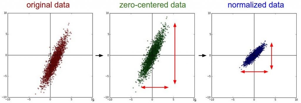
image from: https://www.kdnuggets.com/2018/10/notes-feature-preprocessing-what-why-how.html

This animation shows the feature „frequency of system calls in sequence“ scaled using Z-score normalization for all training sequences.

Before feature scaling the SVM reached an accuracy of 0.86.

from sklearn import preprocessing
scaler = preprocessing.StandardScaler().fit(training_data)
scaled_training_data = scaler.transform(training_data)
scaled_validation_data = scaler.transform(validation_data)
...

After feature scaling the SVM reached an accuracy of 0.87.

Dimensionality Reduction

As mentioned before, not all 520 possible system calls occur in the data. Therefore it would be possible to reduce the size of the feature vector without losing information. Another variant is the PCA. The principal component analysis reduces the number of dimensions by obtaining a set of principal dimensions. Wikipedia summarizes the PCA as follows: “linear mapping of the data to a lower-dimensional space in such a way that the variance of the data in the low-dimensional representation is maximized” [Wikipedia]

Another interesting possibility of dimension reduction is the use of autoencoders. An Autoencoder is a special kind of artificial neuronal network capable of learning a non-linear dimension reduction function. For a very good introduction to autoencoders I can recommend this blog post: Lil’Log.

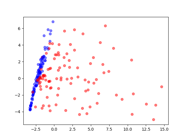
PCA

Visualization of the training data reduced to two dimensions by a principal component analysis. Blue circles are normal behaviour, red ones are attack behaviour.

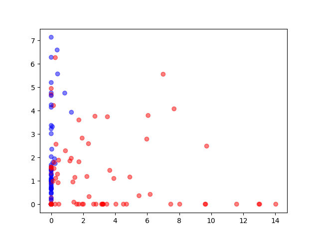
Autoencoder

Visualization of the training data reduced to two dimensions by an autoencoder (520-100-50-25-2). Blue circles are normal behaviour, red ones are attack behaviour.

Reduction to 5 Dimensions with PCA

This animation shows the feature „frequency of system calls in sequence“ reduced to 5 dimensions. scaled using Z-score normalization for all training sequences.

Before dimensionality reduction the SVM reached an accuracy of 0.87.

from sklearn.decomposition import PCA
pca = PCA(n_components=5)
pca.fit(scaled_training_data)
pca_training_data = pca.transform(scaled_training_data)
pca_validation_data = pca.transform(scaled_validation_data)
...

After dimensionality reduction the SVM reached an accuracy of 0.88.

Does it work with an Artificial Neural Network?

I was wondering if this would work just as well with more complex classifiers. That’s why I used the same procedure for a Feed Forward Neural Network (which you can see in the code snippet below).

I came up with the following results:

Support Vector Machine

• raw data as input:
  • accuracy = 0.86
• scaled data as input:
  • accuracy = 0.87
• scaled, pca(5) data as input:
  • accuracy = 0.88

Feed Forward Neural Network

• raw data as input, shape 520-50-50-50-1:
  • accuracy = 0.5 (didn’t learn anything)
• scaled data as input, shape 520-50-50-50-1:
  • accuracy = 0.91
• scaled, pca(6) data as input, shape 6-50-50-50-1:
  • accuracy = 0.93

Looks great, isn’t it? But is there more? Let’s try a convolutional neuronal network (CNN).

Back to the Data

I use the frequency of system calls as input data. From now on I will use the complete sequence instead of the frequency of system calls as input data. In this example the sequences are of different length, with 69.841 system calls in the longest sequence. Since Neuronal Networks have a fixed input size I’ll simply fill the missing positions with zeros.

data = np.array([xi + [0] * (max_length - len(xi)) for xi in data])

With this data as input the CNN scored an accuracy of 0.5, again it didn’t learn anything.

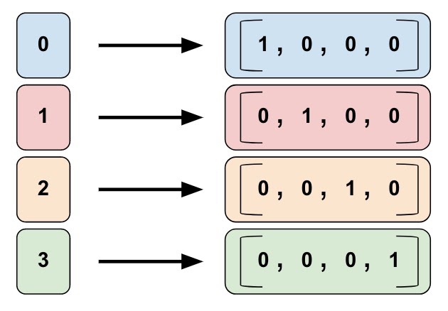
image from: https://www.tensorflow.org/guide/feature_columns

Again to the Data: One Hot Encoding

The system call numbers are categorical data. Such kind of data has to be prepared for a artificial neuronal network. I used so called „One Hot Encoding“ for it. This technique is also called indicator variables. In one hot encoding a category (or in this case a system call) is encoded as a vector of size y where y is the number of unique categories (or system calls). In the data used for this article there are only 26 different system calls used present. Therefore the One-Hot-Encoding vector for one system call is of length 26. In addition to the length of 69.841 system calls for the input sequences the actual input size of the CNN is 26 x 69.841 = 1.815.866 input neurons.

You can see the the used CNN in the code snippet below. I used a kernel size of 78 because this will cover 3 system calls of length 26. The stride was set to 26 so the kernel will move from system call to system call in the input vector.

Using One Hot Encoding the CNN scored an accuracy of 0.97.

Final Thoughts

As can be seen from this example, the results of ML algorithms can be improved by relatively simple methods. I would wish that these preprocessing steps are not skipped so often in papers and are documented accordingly.